Getting Started with scRNA-seq: Post-Sequencing Data Analysis

In this article, we will focus on the final stage of the single cell RNA sequencing (scRNA-seq) experiment: data analysis.

Before diving into the intricacies of analysis, it is important for scRNA-seq novices to understand the single cell library preparation methods. This knowledge is crucial, as technical artifacts that arise during the preparation process can significantly influence the quality control (QC) checks and filters applied to the dataset.

There are multiple approaches for achieving single cell separation. Each method comes with its advantages and limitations, influencing the choice of technology based on experimental needs and resources.

Droplet-Based Technology

Droplet-based technology utilizes a microfluidic system to physically separate cells in a suspension into individual compartments by introducing them into oil droplets. These droplets contain the cells, as well as barcoding beads and reaction reagents needed for reverse transcription and library preparation.

While this method has significantly advanced research in the single cell field, it comes with certain limitations, as it requires specialized equipment, which can substantially increase the cost of experiments. Moreover, due to the need for cells to pass through a narrow microfluidics channel, it is not suitable for profiling large or irregularly shaped cells.

Combinatorial In-Situ Barcoding

A novel strategy using combinatorial in-situ barcoding offers an alternative. This approach involves a fixation and permeabilization of the cells, allowing each cell to act as its own reaction compartment, rather than relying on emulsion droplets.

The process starts with fixed and permeabilized cells placed in a 96-well plate, where RNA is reverse-transcribed using oligo-dT and random hexamer primers. The cells are pooled and randomly distributed into a second 96-well plate, where a second barcode is ligated to the transcripts. This process happens a third time, then the cells are counted and transferred into tubes for lysis, library preparation, addition of a fourth barcode, and sequencing.

Irrespective of the methodology used, after sequencing the user will likely receive FASTQ files from their sequencing core facility or sequencing provider. The standard scRNA-seq data analysis pipeline starts with processing these FASTQ files to generate count matrices, followed by quality control and filtering steps to ensure that only high-quality data is retained during post-processing and analysis.

Understanding FASTQ Files

FASTQ files are text-based files that store sequencing data, containing both nucleotide base calls and their associated quality scores. These files can also include metadata such as details about the sequencing instrument, the read position in the flow cell, lane information and flow cell identifiers.

Most sequencing providers perform this conversion, supplying the necessary FASTQ files for the user’s pipelines.

Process Workflow: From FASTQ File to Count Matrices Generation

FASTQ files primary use is in creating gene count matrices (Figure 1).

Figure 1: Obtaining count matrices entails procuring the FASTQ files and performing a thorough QC.

After processing FASTQ files through a standard scRNA-seq pipeline, count matrix files are generated. These matrices represent the number of counts for every gene across each profiled cell in the experiment. Typically, these matrices are provided in three components:

• Sparse Matrix (MTX file) represents the count data in a compact format.
• Cell Metadata contains barcode information.
• Gene List includes gene names and IDs.

When combined, these files reconstruct the count matrix, offering a comprehensive view of the data.

Key Steps in Processing FASTQ Files

Obtaining count matrices requires several intermediate steps. Users can choose a pipeline that best meets their alignment and mapping needs.

Typically, commercial single cell providers offer a pipeline optimized for their specific single cell methodology. For Parse datasets that would be the equivalent of running the ‘Pipeline’ module in Trailmaker or running split-pipe on your local servers.

Starting with FASTQ files, the first step is a QC check. Tools like FASTQC or MultiQC are often used to visualize sequencing quality and validate the information.

Next, the reads must be aligned to the reference genome of interest—an essential step in the pipeline. Numerous tools are available for alignment, including open-source options like STAR, kallisto, bustools, nf-core pipelines from Nextflow, and others.

Upon completion of alignment steps, count matrices are generated.

Pipeline Selection Considerations

Despite the variety of pipelines available, they share a common characteristic: they are computationally intensive and have specific hardware requirements. Most of these pipelines require a Linux operating system and heavy RAM requirements depending on the size of the sequencing data output.

Processing the data can also be time-consuming, even when using a high performance computing cluster. These requirements can seem overwhelming, especially if lacking access to an HPC or a cloud server.

Fortunately, there are solutions available to address this challenge. Depending on the nature of the data, cloud-based platforms like the Trailmaker platform developed by Parse Biosciences can process FASTQ files.

When count matrices are ready, QC steps ensure the removal of low-quality data points.

Quality control involves filtering out unwanted data, identifying artifacts like dead cells and doublets, and addressing contamination issues to ensure that only high-quality data are retained for downstream analysis.

Some of the most important pitfalls to watch out for in the data and should be included as a standard part of the downstream analysis are the following:

• Background and empty droplets
• Dead or dying cells
• Doublets
• Contaminant cells and ambient RNA
• Batch effects

Removing Background or Empty Droplets

To understand single cell quality control, we must first understand what to expect in an ideal scenario.

For example, in combinatorial barcoding methods each cell is expected to be uniquely barcoded with a low percentage of doublets and minimal free-floating mRNA that could be mistakenly barcoded and retained. In droplet-based technologies, each cell should be encapsulated within a distinct oil droplet, with as few free-floating transcripts as possible.

In less ideal scenarios, multiple cells within a single droplet or barcoded together, as well as droplets containing free-floating transcripts, with or without cells result in barcoded background RNA. Combinatorial barcoding is less susceptible to background issues due to separate in-cell barcoding (Figure 2).

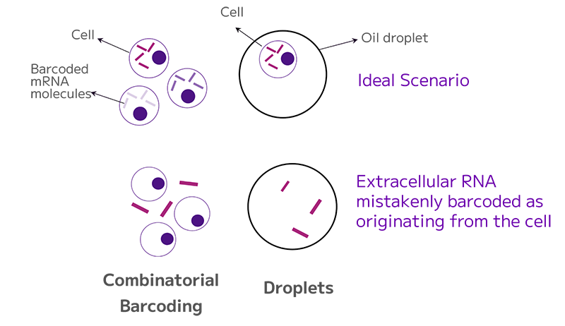
Figure 2: Only the cell’s barcoded RNA should be retained. When free floating RNA is barcoded, it results in background RNA.

To prevent the issue, starting with a cell suspension with minimal debris or damaged cells greatly improves the downstream analysis, saving time during data processing. For a more in-depth discussion on this topic, refer to our previous article on sample preparation.

But if background RNA is present, it can be computationally removed.

One method for filtering data is the classifier filter, which employs a mathematical model to estimate the composition of the dataset. It identifies barcodes that correspond to real cells as opposed to background noise.

A user-defined false discovery rate (FDR) threshold removes barcodes with a high probability of being empty. This method is particularly effective for droplet-based datasets, where distinguishing between real cells and background is crucial.
Tools like knee plots are also helpful for distinguishing biological cells from background.

Knee plot filters allow researchers to apply a hard threshold based on the inflection point visible in the curve, helping to distinguish biological cells from barcodes associated with background.

A good starting point is to set a transcript threshold, such as 200 or 500 transcripts per cell at standard read depth and adjust this based on the biological context and characteristics of the samples.

Identifying Dead or Dying Cells

Another key step in QC is identifying dead or dying cells. As cell membranes become fragile, transcripts begin to leak out, resulting in a lower overall transcript count in the cytoplasm. However, mitochondrial transcripts remain intact within the mitochondria as it is membrane bound. This can lead to a higher fraction of mitochondrial reads after cell lysis and sequencing.

There are two filtering approaches. One is setting a hard threshold based on biology. The second uses the distribution of the mitochondrial read fractions in the dataset.

Mitochondrial read fractions can be utilized to plot the percentage of mitochondrial reads relative to the number of cells or the total transcripts per cell to set appropriate thresholds.

A commonly used threshold is 10–20%. However, this may vary based on cell type – stressed cells may require a higher threshold to avoid excluding important data points, whereas nuclei should have no mitochondrial reads, as mitochondria are absent.

Identifying and Removing Doublets

Doublets occur when two or more cells share the same barcode, which can introduce artifacts in the data. Doublets can arise in both droplet-based and combinatorial barcoding methods, but they are more common in droplet-based technologies due to factors like flow rate adjustments and cell loading density (Figure 3).

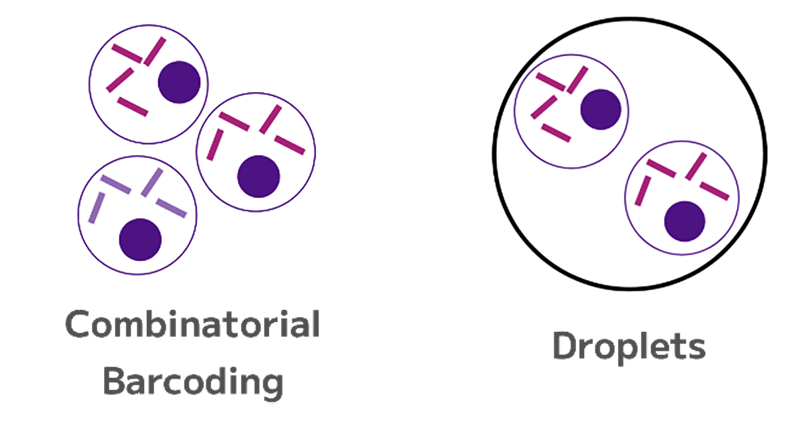
Figure 3: In a doublet, two or more cells have picked up the same barcode or barcode combination.

Several tools are available to identify and remove doublets bioinformatically—Scrublet for Python users, SC DoubletFinder for R users—that have shown strong performance in benchmarking studies.

These tools generate artificial doublet profiles and use scoring systems to assess the likelihood that a cell’s expression profile matches that of a doublet. A key input for these tools is the expected doublet rate, which depends on the chosen methodology and the characteristics of the sample.

Red Blood Cells (RBCs) and Ambient RNA

Contamination is another common challenge, such as the presence of red blood cells (RBCs) in PBMC datasets.

A cluster characterized by many transcripts per cell but few genes per cell may indicate RBC contamination. To remove them, dimensionality reduction techniques like UMAP makes it easier to exclude them from the analysis.

Ambient RNA refers to free-floating transcripts that are inadvertently barcoded alongside intact cells, a problem often seen in droplet-based technologies due to their compartmentalization methods. Tools like SoupX, CellBender, and DecontX can help mitigate ambient RNA contamination and also provide guidance on when to apply them during preprocessing to effectively remove unwanted RNA.

Remove Batch Effect

Batch effects are a common issue in single-cell datasets, as samples are often processed under different conditions, with varying technical factors such as handling personnel, reagents, or even different technologies. These systematic differences can obscure genuine biological variations.

It is advisable to remove these technical differences if they appear on UMAP plots. Data integration is the solution for removing such batch effects.

For data integration and batch effect removal, the appropriate tool will depend on factors like sample variation. For instance, time-course studies with different cell types at each time point need a different tool than studies with consistent cell types across samples.

Tools to consider include Seurat, SCTransform, FastMNN, scVI, and others.

Once count matrices from the FASTQ processing pipeline are obtained and you have applied the required filtering and QC steps discussed in the previous section, the next step is to explore the data by visualizing the data in the form of clusters and generating insights like differentially expressed genes.

Data Normalization and Transformation

Normalization is essential due to the prevalence of zero counts and low gene counts in single cell data. It involves dividing each gene’s expression by the total expression per cell, followed by multiplying by a scaling factor, such as 10,000. This scaling process simplifies further analysis by standardizing expression levels across cells.

Log transformation adjusts the range of gene expression values, making the data more comparable across different cells, especially when dealing with varying transcript levels. Log transformation helps to reduce the impact of highly expressed genes, focusing instead on biologically relevant variations.

Dimensionality Reduction and Clustering

Single-cell datasets contain thousands of genes, but typically only a subset drives the variance observed between different clusters. To capture these key differences, PCA is a common technique used to reduce dimensionality. It is common to retain 30 to 50 principal components, focusing on highly variable transcripts that best represent the diversity in the dataset.

Generating Embedding Plots

Embedding plots like UMAP (Uniform Manifold Approximation and Projection) or t-SNE (t-Distributed Stochastic Neighbor Embedding) visualize cellular clusters.
These plots help to map the reduced dimensions into two or three dimensions, offering a visual representation of the cell populations in the data.

Generally, clustering resolution is adjusted based on the biological characteristics of the dataset, testing different resolution parameters to identify the optimal clustering for the data.

Cluster Identification and Annotation

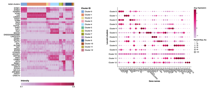
Marker heatmaps are useful for identifying highly variable genes across clusters, aiding in the assignment of cluster identities. Dot plots are also an effective method to visualize gene expression patterns across different clusters (Figure 4).

Figure 4: Marker heatmaps and dot plots enable the visualization of highly dispersed genes, facilitating the assignment of cluster identities.

Popular tools aiding automatic annotation such as Azimuth, CellTypist, and ScType are valuable tools useful in annotating cell types.

Automatic annotation tools are a good starting point for identifying cell types, but they should not be the final step—these methods can be influenced by the quality of training data and how closely the data matches the reference.

Combining automatic annotations with traditional marker-based methods, literature references, and a deep understanding of cell biology can greatly improve annotation accuracy.

Differential Gene Expression (DGE) Analysis

Differential gene expression is a fundamental analysis in single-cell research, providing insights into gene regulation and cell behavior. There are two main approaches.

DGE analysis within a single sample compares cell sets/ clusters within a single sample/ metadata group to identify variations between cell types or states.

DGE analysis across different samples compares the same cell types across multiple samples, such as examining a specific cell type across different conditions or donors.

The scRNA-Seq Analysis Toolkit

Different quality checks and analysis methods are available for single cell data sets, cloud tools or open source.

Cloud-based tools can aid the FASTQ file processing, run QC filtering, and explore the data generating insights.

Indeed, cloud platforms like Trailmaker streamline the analysis workflow, supporting everything from FASTQ file processing to the generation of publication-ready visualizations.

For those who prefer more hands-on approaches, several open-source tools are available: Seurat (R) and Scanpy (Python) are widely used for versatile and in-depth analysis. Bioconductor is a powerful suite of R packages for bioinformatics, and CELLxGENE is a user-friendly platform that simplifies visualization and analysis of single-cell data.

Analyzing scRNA-seq data involves careful preparation, processing, and quality control to ensure reliable results. Understanding the different library preparation methods helps mitigate technical issues.

Key steps include processing FASTQ files to create count matrices, thorough QC to remove artifacts like dead cells and doublets, and addressing batch effects. Data normalization, dimensionality reduction, and clustering help visualize and interpret cell populations. Using tools like Seurat or cloud platforms simplifies these processes and enhances data analysis.

Mastering these techniques allows researchers to draw meaningful insights from complex scRNA-seq data.